The Least Squares Method is a statistical technique used to find a line or curve that best fits a set of points. It is invaluable in statistics, helping us make educated guesses by establishing a few set points in advance.
We can also use the Least Squares Method to translate camera coordinates into robot coordinates. This method helps determine the optimal way to rescale, rotate, and translate the camera’s coordinate system to align perfectly with the robot’s coordinate system.
Transforming camera coordinates to robot coordinates can be done using a Least Squares Method to align both systems accurately by calculating the required transformation parameters.
The general transformation equations are:
xd = a * xp + b * yp + c
yd = d * xp + e * yp + f
Where:
• xd and yd are the robot’s coordinates,
• xp and yp are the camera’s coordinates,
• a, b, c, d, e, and f are the transformation parameters.
To find these parameters, use the following Python script:
import numpy as np
import matplotlib.pyplot as plt
# Input data (camera coordinates)
# [x, y, 1]
A = np.array([
[camera x, camera y, 1], #add more for better results
[camera x, camera y, 1],
[camera x, camera y, 1],
])
# Target data (robot coordinates)
# [x, y]
B = np.array([
[robot x, robot y], #add more for better results
[robot x, robot y],
[robot x, robot y],
])
# Solve the least squares problem
coefficients, _, _, _ = np.linalg.lstsq(A, B, rcond=None)
# Print each coefficient
print("Coefficients:")
print(f"a = {coefficients[0, 0]}")
print(f"b = {coefficients[1, 0]}")
print(f"c = {coefficients[2, 0]}")
print(f"d = {coefficients[0, 1]}")
print(f"e = {coefficients[1, 1]}")
print(f"f = {coefficients[2, 1]}")
# Apply the transformation to the camera coordinates
transformed_coords = A @ coefficients
# Compare the transformed coordinates with the robot coordinates
print("\nTransformed coordinates vs. Actual robot coordinates:")
for i in range(len(B)):
print(f"Transformed: {transformed_coords[i]} vs. Actual: {B[i]}")
# Calculate the Mean Squared Error (MSE)
mse = np.mean((B - transformed_coords) ** 2)
print(f"\nMean Squared Error (MSE): {mse}")
# Calculate the accuracy as a percentage
max_value = np.max(B)
accuracy = 100 - (mse / max_value) * 100
print(f"Accuracy: {accuracy:.2f}%")
# Calculate Euclidean Distance
distances = np.linalg.norm(B - transformed_coords, axis=1)
average_distance = np.mean(distances)
print(f"Average Euclidean Distance: {average_distance:.4f}")
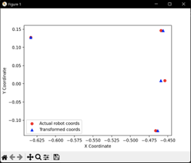
# Plotting the results
fig, ax = plt.subplots()
ax.scatter(B[:,0], B[:,1], c='r', marker='o', label='Actual robot coords')
ax.scatter(transformed_coords[:,0], transformed_coords[:,1], c='b', marker='^', label='Transformed coords')
ax.set_xlabel('X Coordinate')
ax.set_ylabel('Y Coordinate')
ax.legend()
plt.show()
To use the script, you’ll need to insert your camera coordinates and the corresponding robot coordinates into the provided arrays.
Establishing Initial Coordinates:
-
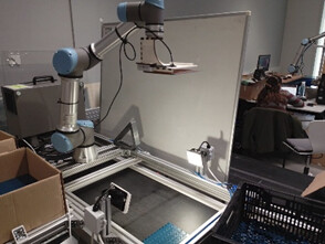
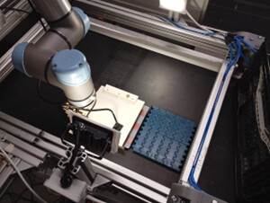
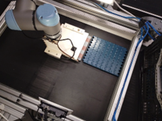
Setup: Create a setup for how your robot will move in your work area. This method assumes your camera is stationary. If the camera is attached to the end of the robot arm, define a capture position for the robot.
-
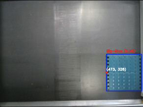
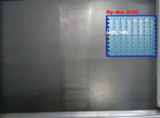
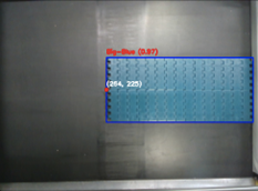
Capture Position: Move the robot to the capture position and check the camera for the item’s coordinates.
-
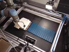
Align Position: Manually move the robot to where it should be if the item is at the captured coordinates. If you have any tool offset setting, make sure it’s consistent and present in this step as well. For better TCP accuracy, get the robot as close as possible to the desired item and capture this TCP
-
Repeat: Capture several sets of coordinates with the item in different positions to improve accuracy. Aim for 7 positions for optimal results.
Example of usage with given coordinates:
# Input data (camera coordinates)
# [x, y, 1]
A = np.array([
    [269, 241, 1],
    [435, 350, 1],
    [269, 110, 1],
    [270, 372, 1],
])

# Target data (robot coordinates)
# [x, y]
B = np.array([
    [-0.45392306201597526, 0.008666534496233558],
    [-0.6332256232813833, 0.12730990848339344],
    [-0.4661438800601707, -0.12857826313800147],
    [-0.45911760805987534, 0.14637253602441908],
])
Here is an example of what you should see after running the script:
Coefficients:
a = -0.0010677615453140213
b = 3.094561948991097e-05
c = -0.17959680557618776
d = 2.482562688915765e-05
e = 0.0010493343791252749
f = -0.2507558317896495

Transformed coordinates vs. Actual robot coordinates:
Transformed: [-0.45936677 0.00881185] vs. Actual: [-0.45392306 0.00866653]
Transformed: [-0.63324211 0.12731035] vs. Actual: [-0.63322562 0.12730991]
Transformed: [-0.46342064 -0.12865096] vs. Actual: [-0.46614388 -0.12857826]
Transformed: [-0.45638065 0.14629948] vs. Actual: [-0.45911761 0.14637254]

Mean Squared Error (MSE): 5.571609920914277e-06
Accuracy: 100.00%
Average Euclidean Distance: 0.0027
You’ll get the a, b, c, d, e, and f coefficients, and the script will test their accuracy. In the plotted results, you’ll want the circles and triangles to overlap for high accuracy. Any alignment discrepancy within three decimal places indicates a highly accurate translation.
Once you have your coefficients, you can use them in a function like this:
    def transform_coordinates(self, xp, yp, zp):
        a, b, c = -0.0010677615453140213, 3.094561948991097e-05, -0.17959680557618776
        d, e, f = 2.482562688915765e-05, 0.0010493343791252749, -0.2507558317896495

        xd = a * xp + b * yp + c
        yd = d * xp + e * yp + f

        return xd, yd